Match List-I with List-II:List-IList-II(A)q = x1α x2β(I)Increasing re…

Match List-I with List-II:

List-I		List-II
(A)	q = x₁^α x₂^β	(I)	Increasing returns to scale
(B)	α + β > 1 in q = x₁^α x₂^β	(II)	Cobb-Douglas production function
(C)	Average fixed cost curve	(III)	‘U’-shaped
(D)	Short run marginal cost curve	(IV)	Rectangular hyperbola

Choose the correct answer from the options given below:

Answer & explanation

Correct answer: option 3

The correct answer is Option (3) → (A)-(II), (B)-(I), (C)-(IV), (D)-(III)

Two items are about the Cobb-Douglas function and two about the shapes of short run cost curves.

List-I	List-II	Reason
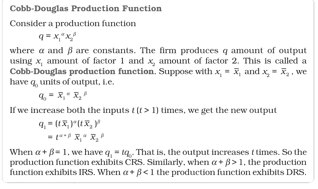
(A) q = x₁^α x₂^β	(II) Cobb-Douglas production function	A function of this form, with powers on the two inputs, is called a Cobb-Douglas production function.
(B) α + β > 1 in q = x₁^α x₂^β	(I) Increasing returns to scale	Raising both inputs t times raises output t^{α + β} times, which is more than t when α + β > 1.
(C) Average fixed cost curve	(IV) Rectangular hyperbola	AFC × output always equals the constant TFC, so the AFC curve is a rectangular hyperbola.
(D) Short run marginal cost curve	(III) ‘U’-shaped	SMC first falls and then rises, because MP first rises and then falls.

NCERT (2026-27): “Cobb-Douglas Production Function … When α + β = 1, we have q₁ = tq₀. That is, the output increases t times. So the production function exhibits CRS. Similarly, when α + β > 1, the production function exhibits IRS. When α + β < 1 the production function exhibits DRS.”

NCERT extract

“Shapes of the Short Run Cost Curves … AFC is the ratio of TFC to q. TFC is a constant. Therefore, as q increases, AFC decreases. When output is very close to zero, AFC is arbitrarily large, and as output moves towards infinity, AFC moves towards zero. AFC curve is, in fact, a rectangular hyperbola. If we multiply any value q of output with its corresponding AFC, we always get a constant, namely TFC.”

“Shapes of the Short Run Cost Curves … Let us now look at the SMC curve. Marginal cost is the additional cost that a firm incurs to produce one extra unit of output. According to the law of variable proportions, initially, the marginal product of a factor increases as employment increases, and then after a certain point, it decreases. This means initially to produce every extra unit of output, the requirement of the factor becomes less and less, and then after a certain point, it becomes greater and greater. As a result, with the factor price given, initially the SMC falls, and then after a certain point, it rises. SMC curve is, therefore, ‘U’-shaped.”